Incremental learning

Incremental learning mechanism endow the neural network to fast learn some new tasks without dramatical performance degeneration on old tasks.

Here I put my understanding about several state-of-the-art paper in this field.

Learning without forgetting

Check here for original paper. This paper gives us a good conclusion about the existing methods on incremental learning (or transfer learning) field. I draw that summary here.

Tuning Categories

Let’s say we have pre-trained backbone network with parameters $\theta_s$ , task-specific FC parameters $\theta_o$ , and randomly initialized task-specific FC parameters $\theta_n$ for new tasks. Based on the different parameters adjustment strategies, we have below categories:

Feature Extraction: $\theta_s, \theta_o$ are unchanged, and only $\theta_n$ will be trained.
Fine-tuning: $\theta_s, \theta_n$ will be trained for the new tasks, while $\theta_o$ is fixed. Typically, low learning rate is needed for avoiding the large drift in $\theta_s$ .
Fine-tuning FC: part of $\theta_s$ - the convolutional layers are frozen, and top fully connected layers and $\theta_n$ are tuned.
Joint Traning: All parameters $\theta_s, \theta_o, \theta_n$ are jointly optimized. This method requires all of training data are avaliable.

Joint training usually can achieve the best performance on both old tasks and new tasks, but its efficiency is not quite desirable. Here is a performance comparison table. (Duplicating indicates copy the previous network and tune it on new task).

Proposed strategy

The design of proposed stratgy (i.e. learning without forgetting) is very intuitive and easy.

The key idea is that before training, it records the output of old tasks on new data. Then it uses these records as an extra regulariation to limit the parameters changing.

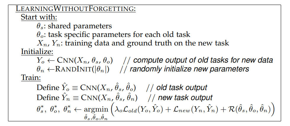
(Conbining this algorithm with above figure (e) can give a good sense of this approach)

$\mathcal{L}_{new}(Y_n, \hat{Y}_n) = -Y_n \log \hat{Y}_n \\ \mathcal{L}_{old}(Y_o, \hat{Y}_o) = -Y_o \log \hat{Y}_o \\ \mathcal{R}(\hat \theta_s, \hat \theta_o, \hat \theta_n) \mbox{ is the common regularization term (e.g. L2-loss)}$

Overcoming catastropic forgetting in neural network

This paper interpret the learning process from probabilistic perspective. Check here for original paper.

First, it says that based on previous research, many different parameter configurations will result in the same performance (this makes sense since neural network has tons of parameters and many of them may be correlated). So the key to avoid catastropic forgetting is to selectively adjust the pre-trained parameters. The more important parameters are, the more slowly they change. The following figure illustrates this idea.

*figure explanation

Elastic weight consolidation (EWC, the name of proposed method) ensures task A is remembered whilst training on task B. Training trajectories are illustrated in a schematic parameter space, with parameter regions leading to good performance on task A (gray) and on task B (cream). After learning the first task, the parameters are at $\theta_A^{*}$ .

If we take gradient steps according to task B alone (blue arrow), we will minimize the loss of task B but destroy what we have learnt for task A.

On the other hand, if we constrain each weight with the same coefficient (green arrow) the restriction imposed is too severe and we can only remember task A at the expense of not learning task B.

EWC, conversely, finds a solution for task B without incurring a significant loss on task A (red arrow) by explicitly computing how important weights are for task A.

Now, how should we determine which parameter is important?

From the probabilistic point of view, given the training data $D$ our goal is to find the best parameter to maximize a posterior (MAP)

$\mathop{\arg\max_{\theta}} p(\theta|D)$

Apply log-transform and Beyas’ rule we have

$\mathop{\arg\max_{\theta}} \log p(\theta|D) = \log p(D|\theta) + log p(\theta) - log p(D)$

Data $D$ can be splitted into dataset $D_A$ (old task) and $D_B$ (new task). Then we re-arrange the objective to There is an assumption: the dataset A and B are independent w.r.t. $\theta$ . In other word, $p(D|\theta) = p(D_A|\theta)*p(D_B|\theta)$

$\log p(\theta|D) = \log p(D_B|\theta) + \log p(\theta|D_A) - \log p(D_B)$

Only the second term $p(\theta|D_A)$ is related with old task. We want to explore the parameter importance information from it.

The Fisher information Fisher information is a way of measuring the amount of information that an observable random variable X carries about an unknown parameter $\theta$ of a distribution that models X. The more information a parameter has, the more influence it can cause to the data X. Check here for the details. is the proper metric to model this.

To calculate the Fisher information, we need to know what kind of distribution $p(\theta|D_A)$ satisfy. However, there is usually no close-form to represent $p(\theta|D_A)$ . Whereby the author assume it satisfies Gaussian distribution, and for calculation simplicity they only consider the diagonal elements in Fisher matrix.

Finally, the objective function is

$\mathop{\arg\min_{\theta}} \mathcal{L}(\theta) = \mathcal{L}_B(\theta) + \sum_i \frac{\lambda}{2}F_i(\theta_i - \theta_{A, i}^{*})^2$

where $\mathcal{L}(\theta) = -\log p(\theta|D)$ , $\mathcal{L}_B(\theta) = -\log p(D_B|\theta)$ , $F_i$ is the corresponding element in Fisher matrix.