Test knowledge

Some basic machine learning knowledge for final test in XMU. These knowledge are related with a lot of topics. I just briefly put them here as a reminder. It can be seen as a complementary with Miscellaneous section.

Searching

Searching is an classic topic in computer science. There are some important searching strategies.

Heuristic searching

The important property in heuristic searching is heuristic function $h(x)$ . The next searching node is selected by $\min f(x) = g(x) + h(x)$ , where $g(x)$ is the cost from root node to current node. This algorithm can be easily implemented via mimimum heap (i.e. queue).

Note that there is a concept, called admissible heuristic, which means that the heuristic function $h(x)$ never overestimates the cost of reaching the goal, i.e. the cost it estimates to reach the goal is not higher than the lowest possible cost from the current point in the path.

Adversarial searching

Adversarial searching is widely adopted in various games. One of the most common strategy is min-max searching with $\alpha-\beta$ pruning.

Min-max Searching Tree

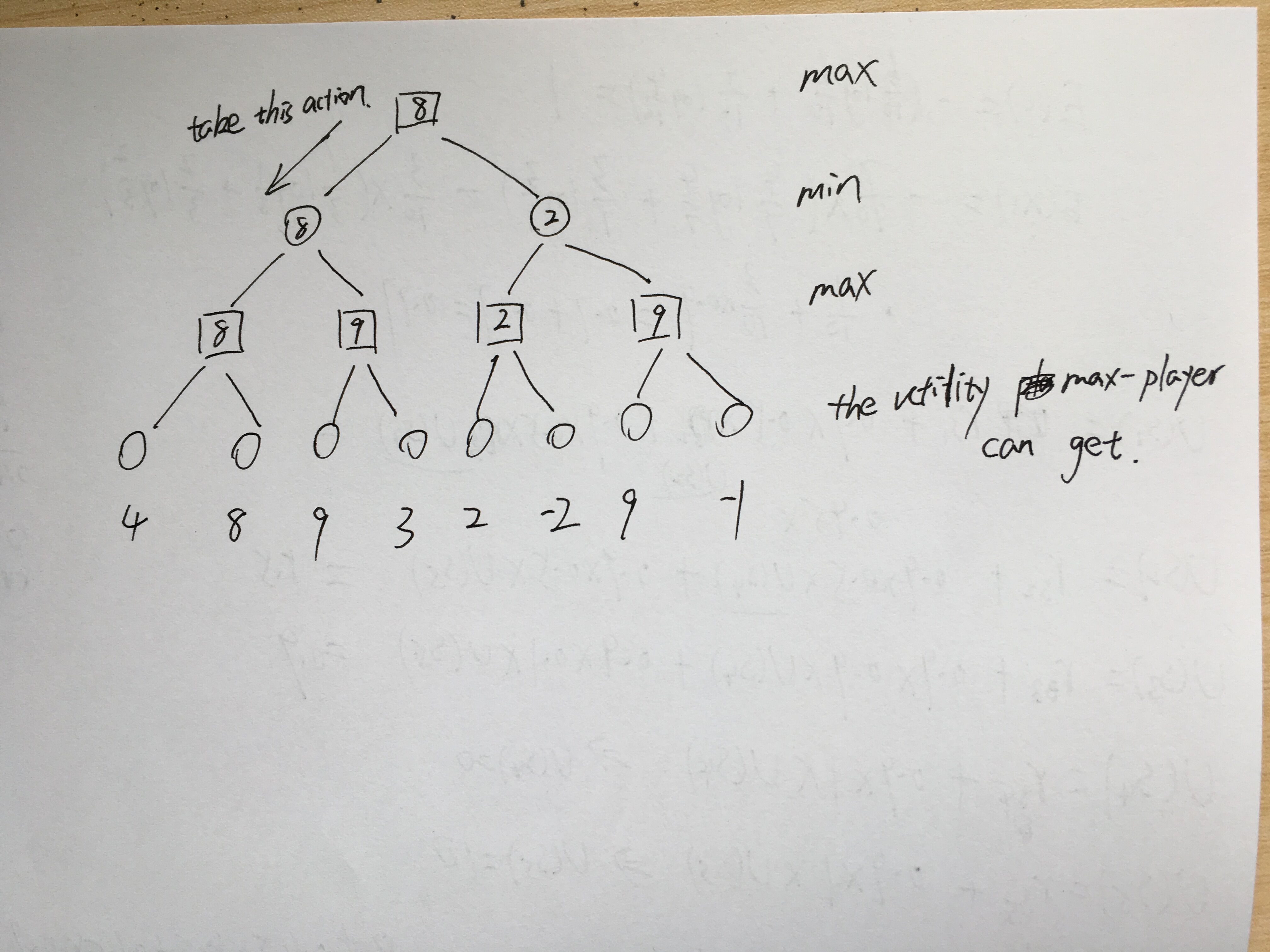
It is a strategy to calculate what action need to be taken for maximizing utility.

The idea of min-max searching is simple. It iteratively pick up minimum or maximum value (i.e. utility) from bottom to top.

An example is showed in below figure.

Alpha-beta pruning

Alpha-beta pruning is stratgy to reduce the searching space in min-max searching tree. Here is the pseudo code for alpha-beta pruning. Check this video for the original code and explanation about alpha-beta pruning.

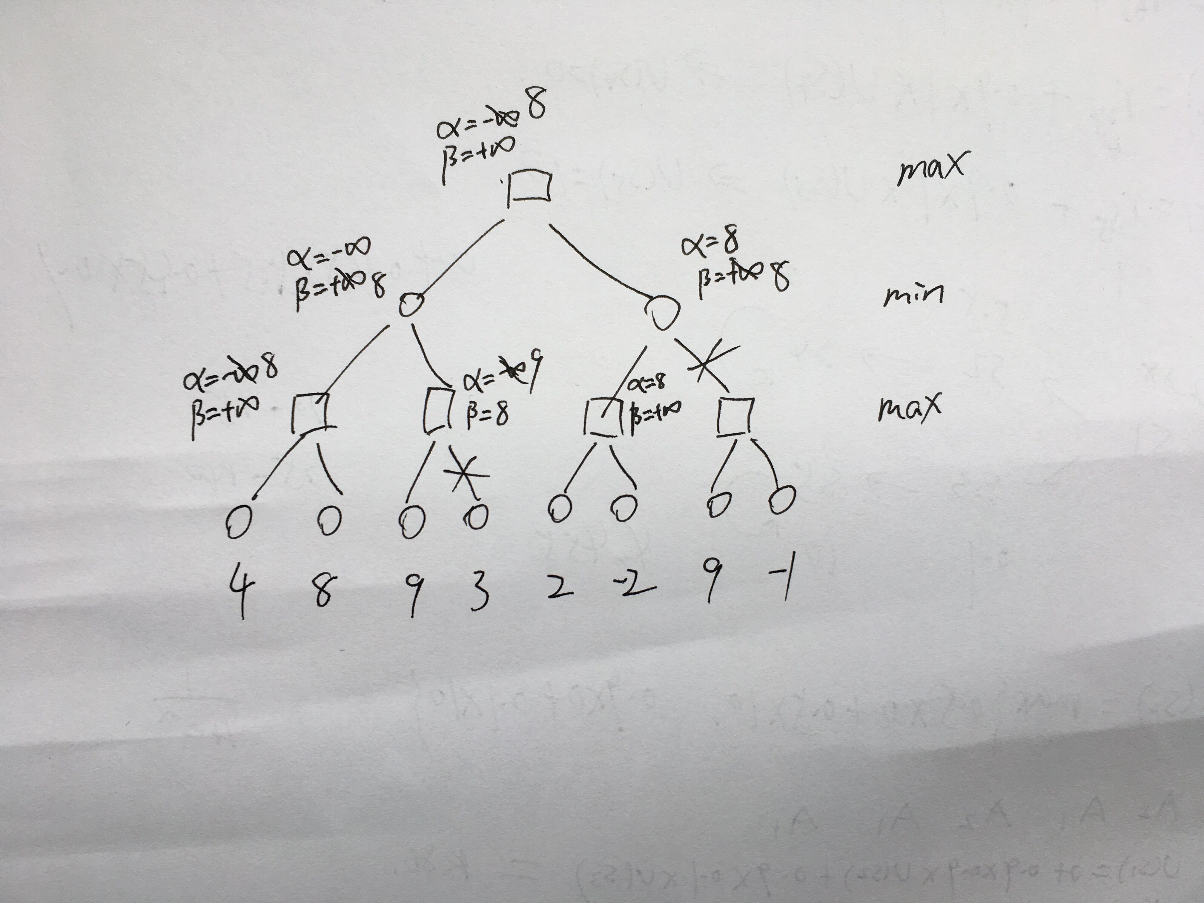
You may get confused since this algorithm is not quite straightforward. I recommend you use below example to run this algorithm by hand so that you can understand how it works.

 
// The MaxVal function. It is called by max player.
// Parameters: s denotes state, a is alpha value, b is beta value.
MaxVal(s, a, b)
{
    if terminal(s) 
    	return U(s);
    v= -infinity;
    for c in next-state(s)
    {
    	temp_v = MinVal(c, a, b);
    	if temp_v > v
    	   v = temp_v;
    	if temp_v >= b
    	   return v;  // The pruning happens. It is also called beta pruning
    	if temp_v > a
    	   a = temp_v;
    }
    return v;
}

// The MinVal function. It is called by min player.
// Parameters: s denotes state, a is alpha value, b is beta value.
MinVal(s, a, b)
{
    if terminal(s) 
    	return U(s);
    v= infinity;
    for c in next-state(s)
    {
    	temp_v = MaxVal(c, a, b);
    	if temp_v < v
    	   v = temp_v;
    	if temp_v <= a
    	   return v;  // The pruning happens. It is also called alpha pruning
    	if temp_v > b
    	   b = temp_v;
    }
    return v;
}

// Driver function to run this algorithm
int main()
{
    v = MaxVal(start_s, -infinity, infinity);
    return 0;
}

There is a simple alpha-beta pruning example I wrote as below picture. I didn’t put the $v, temp\_v$ in draft. With alpha and beta, it is enough for human to figure out whether it should be pruned.

There are some keypoints:

1.The pruning happens whenever alpha>=beta. i.e. Following branches can be ignored.

2.The max node only modifies alpha value and min node only modify beta value.

3.The alpha or beta value in father node will be updated as long as new alpha > alpha or new beta < beta.

Probabilistic Graph Model (PGM)

Generally speaking, PGM consists of two main categories: Beyesian network and Markov network. Both contain a lot of models. I introduce some of them first. If I have time, more content and models will be added in the future. Here is an intuitive introduction.

There is a simple outline:

Probabilistic Graph Model
- Bayesian Network:
  1. Ordinary Bayesian Network
  2. Dynamic Bayesian Network Hidden Markov Model Kalman Fitering
- Markov Network:
  1. Markov Random Field
  2. Conditional Random Field

Bayesian Network (directed acyclic graph a.k.a. DAG )

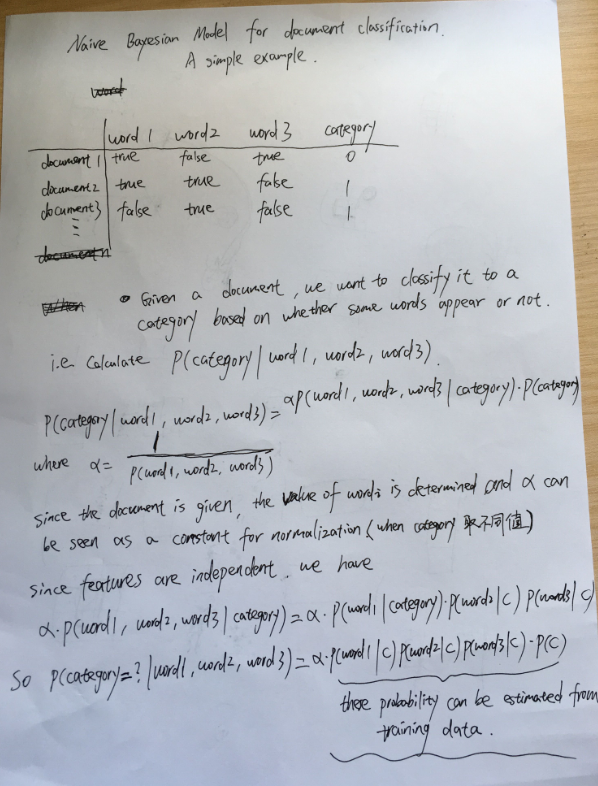
Naive bayesian model

Naive bayesian model assumes all features independently affect the output. For saving time, I wrote an simple example by hand to demonstrate how naive bayesian model can be learned and tested for new task

More general bayesian model

Why we need bayesian network?

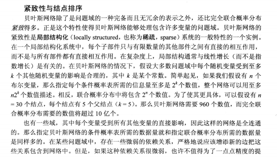
General bayesian network is a simple and elegant tool to represent the relationship among random variables.

The inference methods in bayesian network.

There are two categories methods: accurate inference and approximate inference. In accurate inference, there are some algorithms with the idea of marginalization. However, the accurate inference usually intractable (time complexity is extremely high) when network contains a lot of nodes and edges. In practice, the approximate inference (i.e. sampling methods) is widely adopted. There are two common sampling methods: direct sampling and markov chain monte carlo (i.e. MCMC sampling). Direct sampling method is straightforward: it starts samples from evidence variable, then transmit to other random variables based on conditional probabilities. MCMC method is based on another idea: it starts from a initial state (all random variables have a initial value), then it transmits to next state by modifying one of random variable. Gibbs sampling as a MCMC method is used in bayesian network.

Dynamic Bayesian Network

Unlike ordinary bayesian network, dynamic bayesian network takes time dimension into account. hidden markov model is the simplest and a typical DBN.

Hidden markov model

Hidden Markov Model is a statistical Markov model in which the system being modeled is assumed to be a Markov process with unobservable states. The hidden Markov model can be represented as the simplest dynamic Bayesian network. There are several problems to be solved in HMM.

1.- Given the HMM model and a sequence of observations, how to esitimate the probability of an hidden state. (forward, backward algorithm)

2.- Given the HMM model and a sequence of observations, how to estimate what the most possible hidden state sequences are. (Viterbi algorithm, dynamic programming)

3.- Given the observation data, how to estimate the model parameters. (learning problem, Baum–Welch algorithm)

I’d like to give a detailed introduction about forward-backward algorithm, viterbi algorithm, Baum–Welch algorithm.

Let’s use this picture as a HMM example to introduce these algorithms. The detailed introducation can refer to book 《人工智能一种现代的方法》第三版 15.2章时序模型中的推理

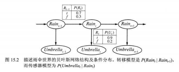
Here $t, f$ denote true or false. It gives transition model (转移模型) and sensor model (传感器模型，also called emission model)

Forward-backward algorithm

Formally, the problem 1 can be represented by $P(X_k|e_{1:t})$ where $X_k$ is the hidden state random variable and $e_{1:t}$ are the evidence/observation variable. Note that the capitalized letter denotes all possible values and lower case letter denotes a specific value.
If $k=t$ , solving $P(X_t|e_{1:t})$ is called filtering . It can be solved by forward algorithm. If $k>t$ , solving $P(X_k|e_{1:t})$ is called prediction . It can be solved by forward algorithm with some more steps iterations. If $k <t$ , solving $P(X_k|e_{1:t})$ is called smoothing . It can be solved by forward-backward algorithm.

When $k=t$ , filtering problem $P(X_t|e_{1:t})$ can be solved iteratively since

$P(X_t|e_{1:t}) = P(X_t|e_{1:t-1}, e_t) = \alpha P(e_t|X_t, e_{1:t-1})P(X_t, e_{1:t-1})$

where $\alpha = \frac{1}{P(e_{1:t})}$ is a constant which can be seen as a normalization term. So we only consider $\alpha$ after finishing calculation and want to normalize $\sum_{x_t} P(x_t|e_{1:t})$ .

Since $e_t, e_{1:t-1}$ are independent, $P(e_t|X_t, e_{1:t-1}) = P(e_t|X_t)$ . On the other hand,

$P(X_t, e_{1:t-1}) = \sum_{x_{t-1}} P(X_t, x_{t-1}, e_{1:t-1}) = \alpha \sum_{x_{t-1}} P(X_t|x_{t-1}, e_{1:t-1})P(x_{t-1}|e_{1:t-1})$

The $\alpha$ here can be ignored too. Because $X_t, e_{1:t-1}$ are independent (Markov property, only $X_t, e_t$ are dependent), we have $P(X_t|x_{t-1}, e_{1:t-1})=P(X_t|x_{t-1})$ .

Finally, we have

$P(X_t | e_{1:t}) = \alpha P(e_t|X_t) \sum_{x_{t-1}} P(X_t|x_{t-1})P(x_{t-1}|e_{1:t-1})$

The first and second terms $P(e_t|X_t), P(X_t|x_{t-1})$ are given, and $P(x_{t-1}|e_{1:t-1}$ is the result in previous time. So we can iteratively solve $P(X_t, e_{1:t})$ from initial state $P(X_0)$ .

Once we get $P(X_t| e_{1:t})$ , the prediction problem (i.e. $k>t$ ) can be easily solved by

$P(X_{t+1} | e_{1:t}) = \sum_{x_{t}} P(X_{t+1}|x_{t})P(x_{t}|e_{1:t})$

We can iteratively reach $P(X_{t+n}|e_{1:t})$ via above formulation.

When $k < t$ , the smoothing problem can be formulated as below

As we can see, the first term $P(X_k|e_{1:k})$ can be solved by above formulation (i.e. forward algorithm).

For the second term $P(e_{k+1:t}|X_k)$ , we have

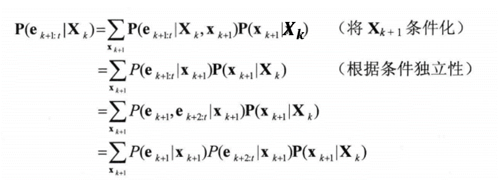
Finally, the first and third term are given and the second term is the iteration term i.e. if we have calculated $P(e_{k+2:t}|X_{k+1})$ , then $P(e_{k+1:t}|X_{k})$ can be calculated via above equation. This is the backward algorithm.

Obviously, we must apply forward and backward algorithm simultaneously to solve the smoothing problem.

An example

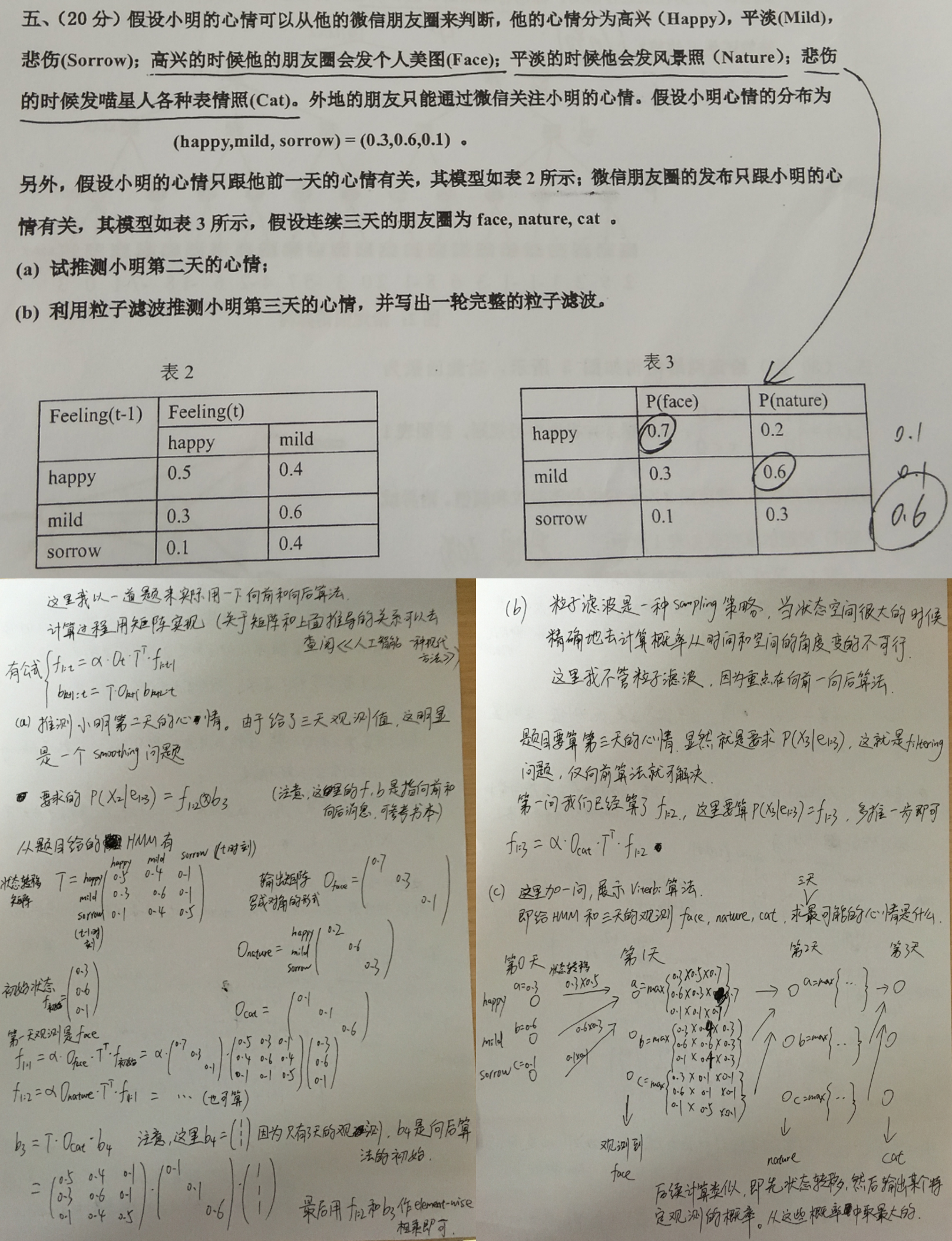
Viterbi algorithm

Viterbi algorithm is for the second problem which can be formulated as below.

Obviously, this formulation is also an iterative algorithm which is quite similar with forward algorithm except it selects the maximum value instead of sum.

A Viterbi algorithm calculation example has been showed in above picture, the question (c).

Baum–Welch algorithm

TODO

Markov Network (undirected graph)

Markov Random Field

Conditional Random Field

Decision Tree

The key concept is information gain (信息增益). In ID-3 algorithm, it uses information gain to decide what property/feature is used for branch generating.

There are also other variants like C4.5 and CART tree.

C4.5 is very similar with ID-3 algorithm and it uses the information gain ratio instead of information gain to build decision tree. The information gain ratio relieves the bias drawback (the features with more possible values are prone to high information gain) in information gain.

CART (classification and regression tree) can simultaneously handle classification (discrete values) and regression (continuous values) problems. It usually builds tree by minimizing Gini index for classification and by minimizing square error for regression. You can search for some examples when coming across this algorithm.

Neural Network

Only back propogation algorithm in multilayer perceptron (MLP) is considered in test.

What I want to emphasize here is that the gradient backprop cannot be calculated by using matrix directly. In matrix calculation, it has a lot derivatives of vector w.r.t. matrix. You should be careful when applying chain rule.

(The derivative of vector w.r.t. matrix is a hyper-matrix and the meaning of elements in hyper-matrix need to be carefully maintained. In fact, I have tried and the gradient calculation cannot be simplified by using vector/matrix. Plain scalar formulation is even better.)